Graphing MDOF Systems
In the Vibrations section of my website I have a graph of a MDOF (Multiple Degree of Freedom) system's frequency response plot and an explanation of how to graph a SDOF in MATLAB. Well someone recently sent me an email asking if they could help them graph a MDOF system. Here is the one on SDOF and below I will explain how to graph a MDOF system.
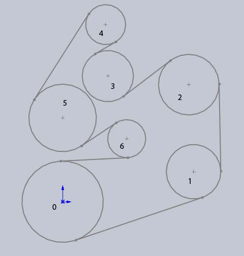
The system that I will be using for this example will be the serpentine belt from an old Ford engine. Solving this system was a part of one of my assignments in Vibrations class. I won't go into the details of this specific system, I'm assuming that you already have your system set up (skip ahead if you do). If you don't have an example of a MDOF system then you can use my code to set up a system. If you don't understand how a MDOF system works you should read more about MDOF systems first because I will not be explaining their basic concepts in this guide.
This system can be defined using the following script file and function file. The script file begins with the following system definitions.
%7DOF pulley system
%input parameters
mass = .2663; %kg, mass of pulley on tensioner spring
J = [0 41.5 13.1 2.63 42.1 17.6 2.08]/10000;  %kg m^2, rotational inertias
r = [81.25 64.5 70.60 -41.15 30 67.5 -38.1]/1000; %m, radii of pulleys
x = [0 261.5 252 90.3 86 0 128]/1000; %m, x location of pulleys
y = [0 60 234 251.1 354 167.5 126]/1000; %m, y location of pulleys

EA = 65000; %N
kT = 9340; %N/m, stiffness of tensioner spring, assumed to be linear

%frequency parameters for graphing
Ldiv = 10; %increment for omega in rpm
Lom = 3000; %max omega in rpm
Then all of this information gets put into the MDOFpulley() function like this:
%response plot
plotOn = 1; %shows plot
[wnrpm,V,Amat,list] = MDOFpulley(J,r,x,y,mass,EA,kT,Ldiv,Lom,plotOn);
This function takes the system information and calculates the lengths of the pulley sections and then creates the equivalent mass, equivalent damping, and equivalent stiffness matrices.
function [wnrpm,V,Amat,list] = MDOFpulley(J,r,x,y,mass,EA,kT,Ldiv,Lom,ploton)
%list = {[lo1,lo2],[EA,kT],J,r,x,y} this gives all the important parameters
%in a large list

    %solve for Lengths
    L = [0,0,0,0,0,0,0];

    n = 1;
    while n <= 7
        if n==7;
            L(n) = ((x(1)-x(n))^2 + (y(1)-y(n))^2 - (r(1)-r(n))^2)^(1/2);
            n = 8;
        else
            L(n) = ((x(n+1)-x(n))^2 + (y(n+1)-y(n))^2 - (r(n+1)-r(n))^2)^(1/2);
            n = n+1;
        end
    end

    k = EA./L;

    %create stiffness matrix
    keq1 = [(k(1)+k(2))*r(2)^2, -k(2)*r(2)*r(3), 0,0,0,0,0];
    keq2 = [-k(2)*r(2)*r(3), (k(2)+k(3))*r(3)^2, -k(3)*r(3)*(-r(4)),0,0,0,0];
    keq3 = [0, -k(3)*r(3)*(-r(4)), (k(3)+k(4))*(-r(4))^2, -k(4)*(-r(4))*r(5),0,0,0];
    keq4 = [0,0,-k(4)*(-r(4))*r(5), (k(4)+k(5))*r(5)^2, -k(5)*r(5)*r(6),0,0];
    keq5 = [0,0,0, -k(5)*r(5)*r(6),(k(5)+k(6))*r(6)^2, -k(6)*r(6)*(-r(7)),...
		(k(6)*r(6))*(x(6)-x(7))/L(6)];
    keq6 = [0,0,0,0,-k(6)*r(6)*(-r(7)),(k(6)+k(7))*(-r(7))^2 ,...
		-(k(6)*(-r(7))*(x(6)-x(7))/L(6))-(k(7)*(-r(7))*(x(7)-x(1))/L(7))];
    keq7 = [0,0,0,0, k(6)*(x(6)-x(7))*r(6)/L(6), ...
		-(k(7)*(x(7)-x(1))*(-r(7))/L(7)) - (k(6)*(x(6)-x(7))*(-r(7))/L(6)),...
		(k(7)*(x(7)-x(1))*(x(7)-x(1))/(L(7)^2)) + ((k(6)*(x(6)-x(7))^2)/(L(6)^2)) + kT];

    keq = [keq1;keq2;keq3;keq4;keq5;keq6;keq7];

    %adjust intertias, J = (mr^2)/2
    rorig = [81.25, 64.5, 70.60, -41.15, 30, 67.5, -38.1]/1000;
    for i = 1:6
        J(i) = (J(i)/((rorig(i)^4)))*(r(i)^4);
    end

    %create mass matrix
    meq = [];
    for i = 1:6
        meq(i,i) = J(i+1);
    end
    meq(7,7) = mass;

    %create damping "matrix", no damping for this problem
    ceq = 0;
Now the function takes these mass, damping, and stiffness matrices and calculates the natural frequencies and mode shapes of the systems. Most of the calculations are done with MATLABs built-in polyeig function. The rest of the code just extracts the important information.
    [Q,lambda] = polyeig(keq,ceq,meq);
    %natural frequency = imaginary component
    lambda2 = imag(lambda);

    %extract only positive lambdas
    lambda3 = [];
    n = 1;
    %zeros = 0
    for i = 1:length(lambda2)
        if lambda2(i) > 0
            lambda3(n) = lambda2(i);
            n = n+1;

        end
    end
    %natural freq in RPM
    wnrpm = lambda3./(2*pi)*60*(1/3);

    %extract mode shapes from eigenvectors
    Q2 = [];
    n = 1;
    for i = 1:(length(Q)/2)
        Q2(:,n) = Q(:,2*i-1);
        n = n+1;
    end
    Q3 = abs(Q2);
    V = Q3;

    for i = 1:length(Q3)
        maxQ3 = max(Q3(:,i));
        Q3(:,i) = Q3(:,i)./maxQ3;
    end
    %mode shapes for each pulley at each frequency
    V = Q3;
This is the important part if you already have your own system. First we make the forces matrix that just states which pulleys have a force applied to them and what are the strength of each force relative to the others. In my case I just said that pulley 1, 6, and 7 all had an equal force of magnitude 1. Then make two empty matrices that will store all of the magnitude responses for each frequency that you want to graph. Then run it through a for-loop that finds these response magnitudes.
    %MDOF frequency response
    forces = [1;0;0;0;0;1;1];
    Amat = zeros(7,Lom/Ldiv+1);
    omegavector = zeros(1,Lom/Ldiv+1);

    n = 0;
    for omega = 0:Ldiv:Lom
        A = ((-(omega/60*(2*pi)*3).^2.*(meq) + (sqrt(-1))*(omega/60*(2*pi)*3).*(ceq) + (keq))^-1)*(forces);
        n = n+1;
        omegavector(n) = omega;
        A = abs(A);
        Amat(:,n) = A;
    end
My test frequencies (omega) happen to be RPM values, but if you were using normal rad/s instead then your magnitudes should be written like this:
%if the input frequencies were in rad/s...
for rads = 0:Ldiv:Lom
    A = (  (  -rads.^2.*(meq) + (sqrt(-1))*(rads).*(ceq) + (keq)  )^-1  )*(forces);
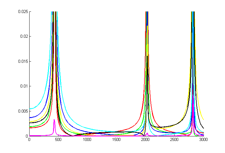
Now we just need to plot our magnitudes stored in 'Amat' vs. our test frequencies stored in 'omegavector'
    figure()
    clf
    hold on
    axis([0, Lom, 0, .025])
    if ploton >= 1
        plot(omegavector,Amat(1,:),'r','Linewidth',2)
        plot(omegavector,Amat(2,:),'g','Linewidth',2)
        plot(omegavector,Amat(3,:),'b','Linewidth',2)
        plot(omegavector,Amat(4,:),'c','Linewidth',2)
        plot(omegavector,Amat(5,:),'y','Linewidth',2)
        plot(omegavector,Amat(6,:),'k','Linewidth',2)
        plot(omegavector,Amat(7,:),'m','Linewidth',2)
    end
Here is the final graph zoomed in on the first two natural frequencies. Also, remember that we used abs() to calculate the magnitude of our frequency response. Besides magnitudes there are also phase shifts to take into consideration. I left damping in this system as ceq = 0 but we could introduce damping into the system. If we did this the problem becomes more complicated, so for now I'm going to leave out a discussion of damping.