PID Controller - MATLAB (Guide)

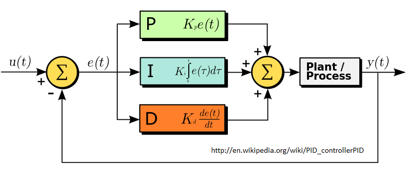
A PID controller takes a setpoint value as an input and uses feedback from a dynamic system to control that system. For example, if the current position of a device is at x = 1 inch and you set the setpoint to 1 then you have reached equilibrium and nothing needs to happen. If you then change the setpoint to 3 then the system calculates an error of 3 - 1 = 2 inches. This error value then goes through the PID (Proportional, Integral, Derivative) controller which then gives a command to move the device. It is important to set the gain values for P, I, and D to be values that create a desirable output from the PID controller. You can do the math or use a PID tuning algorithm when you have a specific task you are trying to solve. However, in order for me to get a better sense of what can happen, I thought it would be interesting to experiment with some different scenarios that a PID controller might encounter.

I would like to eventually turn this page into an interactive graph. Sometime in the future I will get around to creating that. For now I just have various MATLAB graphs with explanations.

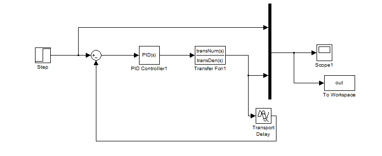
Simulink Model

You can download the MATLAB code and the Simulink Model that I am using do to this testing. The Step block serves as a change from 0 to 1 in the setpoint at t=1 second. The next block takes the setpoint minus the system output to find the current error. This error feeds into the PID which then feeds into the system. The system is simulated by a Transfer Function block. The Transport Delay isn't being used at first (delay=0). The Scope can be used to see a graph of the output and the To Workspace block is used to output to the MATLAB script file.

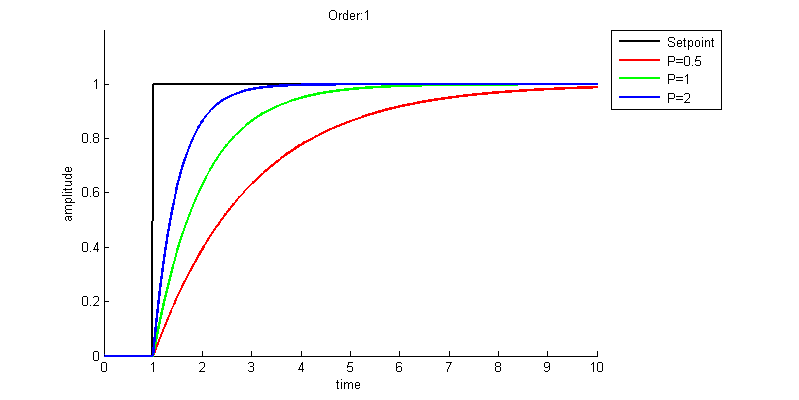
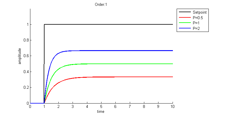
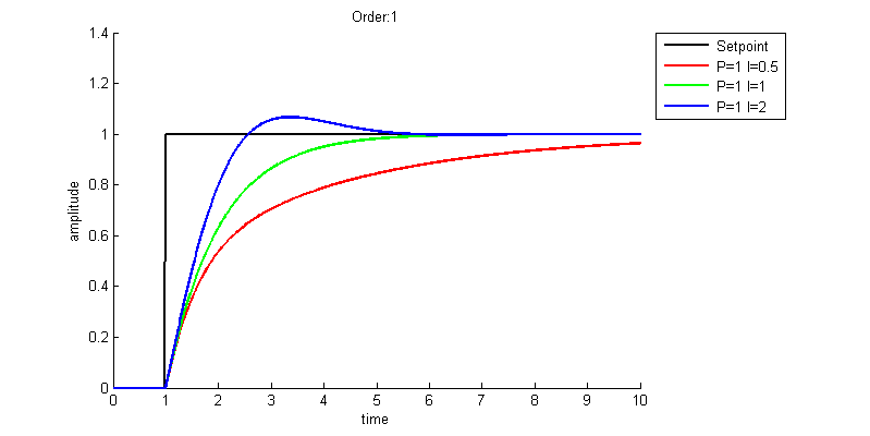
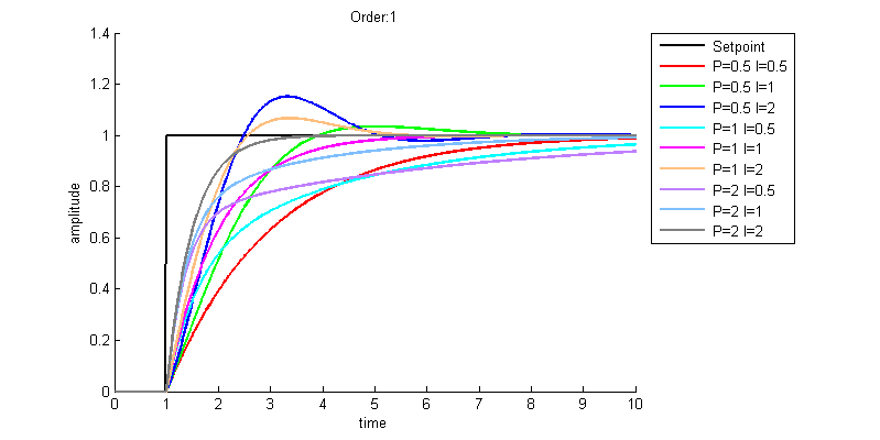
1st Order (1r + 0) | P Only

This is a very simple 1st order system that doesn't "push back" because it has no 0th order term. We can see that in this scenario the PID works exactly as expected. A higher P value increases the speed at which the system reaches its setpoint.

1st Order (1r + 1) | P Only

Now this 1st order system has a 0th order term. This is probably a more realistic situation and we can see that proportional only just doesn't cut it. This result is known as droop and will often occur in systems that are proportional only. This response may seem counter-intuitive at first

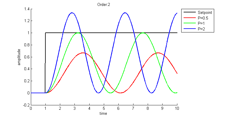
2nd Order (1r^2 + 0r + 1) | P Only

The system has now changed to 2nd order but is still using a P only controller. This 2nd order system has no 1st order damping term and therefore the output continues to oscillate indefinitely. It is unlikely that a real system would have zero damping like this.

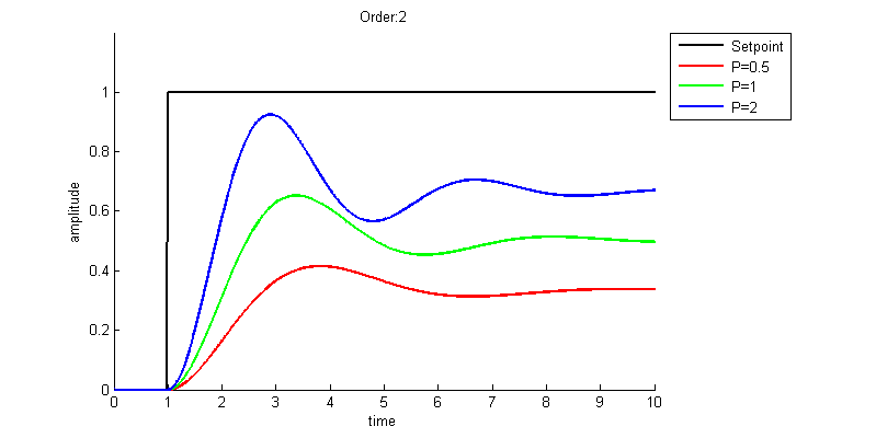
2nd Order (1r^2 + 1r + 1) | P Only

Now the system has a damping term and we can see that the droop problem is still there. Let's add some Integral control to help with droop.

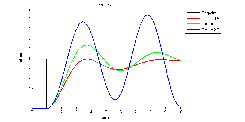
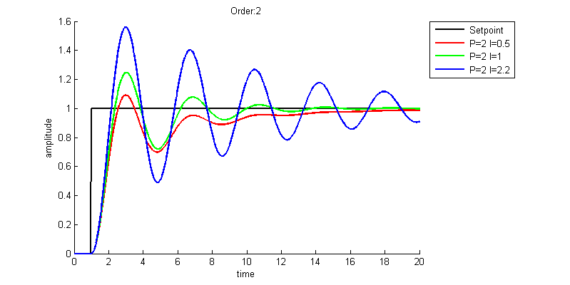
2nd Order (1r^2 + 1r + 1) | P and I

This PI controller now takes care of the droop and gets near the setpoint pretty quickly. However we can see that if we set our integral gain too high we can introduce an instability into the system.

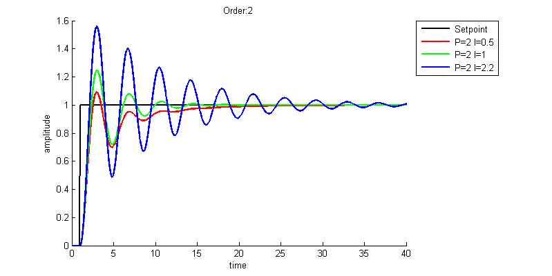
Getting rid of this instability was as simple as increasing the P gain from 1 to 2. I've also changed the scale of the x-axis to include 20 seconds of time. Although the I=2.2 (blue) setup is now stable it's clear that the I=1 (green) setup is far superior. You will see that the I=1 (green) is significantly better if you extend out even further in time.

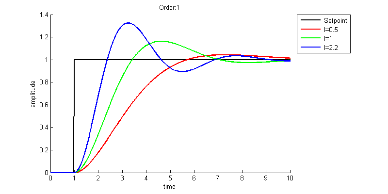
1st Order (1r + 1) | I Only

Let's go back to 1st order and examine a system with Integral only. This seems to work pretty well.

1st Order (1r + 1) | P and I

After adding P back in have we made it any better? The higher Integral values seem to have both significantly improved the time it takes for the system to settle on the setpoint value. The green and blue lines look to be about equal so does it matter which setup we choose if this would be our typical operation conditions? Maybe overshooting causes damage to the system. In that case we may even pick the red setup if it was extremely important to not overshoot.

It seems as though a high P and high I (gray) is the ideal setup. Also the system seems to only overshoot when P < I.

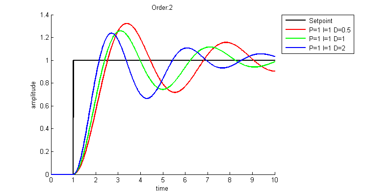
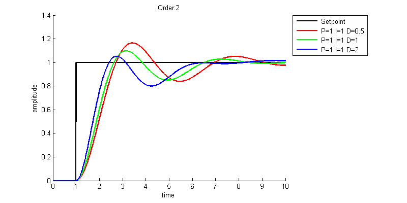
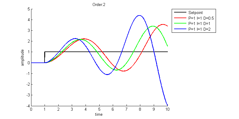
2nd Order (1r^2 + 1r + 1) | P, I, and D

D essentially resists change. The faster the system is changing the harder it resists. This seems like it could decrease the overshoot of a PI system, but that isn't always the case. D control amplifies noise, sometimes with very extreme spikes. Because of this PID controllers often times do not use D control as a PI solution is acceptable. Another alternative is to filter the signal going into the D part of the controller. In MATLAB the filter value 'N' is now set to a coefficient of 1.

We can see with this setup that the D control does a good job of decreasing the overshoot and getting the system to its setpoint quicker.

Additional aspects to consider

Often when tuning a PID there are other certain constraints to consider. Like I mentioned in a previous section, is the device allowed to overshoot? In that case maybe we need to focus less on getting the output to quickly settle on the setpoint and focus more on preventing overshoot. Is there a max acceleration or max velocity constraint on the device? We could place limits on our controllers outputs to satisfy these velocity or acceleration constraints. Additionally the system may have a response lag that prevents the controller from acting the way you would theoretically expect it to act. Lag can often be the cause of instability in a system.

For example take this case of a 2nd Order System(1r^2 + 1r + 1) with a PID controller that has a 1 second delay in the feedback loop. The system now has an unstable response to the step function.

But if we reduce the same system down to a 0.2 second delay the system is now more stable, but definitely less stable than before when the system had no lag.