Writing High-Speed MATLAB (and Python)
Contents
Basic Computer Tricks
Understanding how computers work is fundamental to understanding how to write optimized code. The advice contained in this section will generally apply to all programming languages.
1) Pre-allocate your arrays (~ 100-3000 x faster)
If you have a small array like a 5 x 5 matrix then pre-allocation won't make any difference. However With large array sizes not pre-allocating will have disastrous consequences if you want your program to be fast. Let's start with a simple for-loop from i=1 to i=100000. Each time through the loop you want to assign the i-th spot of an array to the value of the i*2.
NOTE: Remember not to use the variable 'i' or 'j' in your for-loops if you are using complex numbers!
for i = 1:100000
    a(i) = i*2;
end

b = zeros(1,100000); %<--- this is the important pre-allocation code
for i = 1:100000
    b(i) = i*2;
end
Because the length of the 'a' array was never specified MATLAB has to continue to allocate more space for storing the array as the array grows in size. The loop with the 'b' array on the other hand is pre-allocated to a specific size before the loop begins. The 'a' array loop takes a whopping 18000 ms and the 'b' loop only takes 6 ms (3000 times faster). If we reduce the array size down to 10K instead of 100K the difference is not as noticeable but still quite significant at 67 ms for the non pre-allocated and 0.63 ms (100 times faster) for the pre-allocated. By the way, if you don't know how to time your MATLAB code you can write your loop to look like the following:
tic %Starts the timer
b = zeros(1,10000);
elapsed = toc; %Records the time since tic was called, but the timer keeps going
fprintf('%f | Zero Preallocation |',elapsed)
for i = 1:10000
    b(i) = i*2;
end
elapsed = toc; %Once again this records the time since tic was called, and the timer keeps going
fprintf('%f | Zeros with Indexing\n',elapsed)
2) Access your multi-dimensional arrays by row, not by column (~ 1.4 x faster)
Did you know that it is quicker to access the elements of a multi-dimensional array by changing the row index rather than the column index? It isn't much faster, but it is a little bit faster and there is a very good reason for it. When a value is stored in an array it has to be given a specific spot in the memory with a specific address so that the computer knows where to find it. Imagine a mailman delivering mail on a street while he's driving in a mail-truck. The houses on the one side of the street are given the addresses 1001, 1002, 1003, 1004, and 1005 and on the other side of the street they have the addresses 1006, 1007, 1008, 1009, 1010. This is like a 5 x 2 array with values of any number, remember that the values don't matter because we are only talking about the addresses right now. So naturally it will be faster for the mailman to drive down one side of the street while delivering to houses 1001, 1002, 1003, 1004, and 1005. Then he should drive back down the street and deliver to 1006, 1007, 1008, 1009, 1010. This is like asking MATLAB to drive down the array by changing the row index. Just as the mailman with his mailtruck is naturally set up to access a neighborhood in a certain pattern a computer is also set up to naturally access an array in a certain way.
a = rand(1000);
b = a;

tic
for i = 1:1000
    for j = 1:1000
        a(i,j) = a(i,j)*2; %This line is the only difference: (i,j)
    end
end
elapsed = toc;
fprintf('Change Column: %f \n',elapsed)

tic
for i = 1:1000
    for j = 1:1000
        b(j,i) = b(j,i)*2; %This line is the only difference: (j,i)
    end
end
elapsed = toc;
fprintf('Change Row: %f \n',elapsed)
The differences between these two loops are subtle but the second loop only takes 58 ms whereas the first loop takes 78 ms. Keep in mind that in some other programming languages accessing by column might be faster than accessing by row, it just has to do with the way that specific language decides to assign addresses.
3) Reshape and Sort (~ 1.25-2 x faster)
These are really two seperate things but I'm going to put them together because I will demonstrate with a situation that combines both methods. Let's say you have a 1000 x 1000 image matrix where each spot in the matrix represents a pixel in the image matrix. Each one of these pixels contains a random value from 0 (black) to 1 (white). In this case let's apply a threshold to every pixel and keep track of how many pixels are > 0.5 and how many pixels are < 0.5 to see if there are more dark pixels or more light pixels:
a = rand(1000); %1000x1000 image of randomly generated pixels

c1 = 0; %number of pixels counted so far that are closer to 1
c0 = 0; %number of pixels counted so far that are closer to 0

tic
for i = 1:1000
    for j = 1:1000
        if a(j,i) >= 0.5
            c1 = c1+1; % pixel is closer to 1
        else
            c0 = c0+1; % pixel is closer to 0
        end
    end
end
elapsed = toc;
fprintf('Normal: %f \n',elapsed)
These two for-loops currently take about 15 ms. In a lot of cases you will want to keep your 1000 x 1000 image as a 1000 x 1000 matrix, but in this case we no longer care where each pixel is located, we only care about the value of the pixel. Because of this we can reshape our image:
a = rand(1000);
b = reshape(a,[],1); %reshape 'a' such that 'a' is an N x 1 matrix; where N calculated for you

c1 = 0;
c0 = 0;

tic
for i = 1:1000
    if b(i) >= 0.5
        c1 = c1+1;
    else
        c0 = c0+1;
    end
end
elapsed = toc;
fprintf('Reshaped: %f \n',elapsed)
After reshaping our matrix into a 1-D array the loop now only takes 12 ms. We've cut the time a little, the only problem is that we didn't include the reshaping into our time. That's okay though, turns out that after adding the reshaping function under the timer is fast enough to keep us around 12 ms. Now here's a crazy idea, what happens if we then sort our 1-D array before running it through the loop?
a = rand(1000); %
b = reshape(a,[],1);
c = sort(b); %sort 'b' from low to high values

c1 = 0;
c0 = 0;

tic
for i = 1:1000
    if c(i) >= 0.5
        c1 = c1+1;
    else
        c0 = c0+1;
    end
end
elapsed = toc;
fprintf('Sorted: %f \n',elapsed)
This sorting now has taken us down to just 7 ms. What's happening here? Why should it matter if the array is sorted or not? This is due to something called Branch Prediction. A simple explanation for this is that when the processor gets to an if-statement it has to stop and decide which branch of instructions it has to use. Once it has this figured out it then has to load this branch and execute it. What if instead the processor could tell that an if-statement was coming up and then guessed at which branch it would end up having to go down? If it guesses correctly it doesn't have to sit around and wait, but if it guesses wrong then it does have to sit and wait to load the next branch. So if the processor notices that the if-statement almost always evaluates to 'true' then it should keep pre-loading the 'true branch'. In this case when we sort our data we give the processor a huge string of falses and then a huge string of trues.
Unfortunately in this situation if you include the time it takes to sort the array then the program will be slower this way. Because the sorting is a one-time thing we could find an advantage if we had to re-use this sorted array repeatedly. It would be easy to create a more complex situation where sorting would significantly decrease the amount of time required.
4) Variable types (important on GPUs, PICs/Arduinos, and other languages like Python)
MATLAB is a language written so that you don't need to understand much at all about variable types. Variable types are very important in other programming languages, however in MATLAB numbers are automatically assumed to be a double precision floating point (64-bit). There is also single precision floating point (32-bit), and integers that come in the 8-bit, 16-bit, 32-bit and 64-bit variety, with the additional option of being unsigned (always positive). So in summary when you are using MATLAB on a modern day computer you won't need to worry about variable types, you will see barely any increase by using single precision instead of double precision (about 10% speed-up). If instead you are using an Arduino or other PIC you will want to pay attention to these kinds of things. Types will also be important in section 6 when I talk about using a GPU. So in case you care about this 10% decrease in time (and to get you prepared for using the GPU) here it is...
%64-bit, more precise, this is the default type
bDP = double(zeros(1,1000000)); %Allocated as DP using double()

%32-bit, less precise but still very reasonable precision
%Slightly faster on the CPU, much faster on a GPU
bSP = single(zeros(1,1000000)); %Allocated as SP using single()

%Or let's say you wanted the values to only go between 0 and 255
%But be careful, this will slow MATLAB down a little bit
%However on a PIC/Arduino using uint8 should speed things up if you only need 0 - 255
bInt = uint8(zeros(1,1000000)); %Allocated as unsigned 8-bit integers using uint8()
Parallelization / Vectorization
Parallelization is the idea that if you can divide your program into sections of code that can be run at the same time then the computer can send these parallel sections of code to different cores on a CPU/GPU or to several different CPUs on a networked cluster of computers. Parallelization isn't always an option though, consider again the Bio-Kinectics problem I was discussing in the introduction. In this problem there are 4 parameters that are input into the system. For testing purposes we are constraining these 4 parameters to take on all integer values between 1 and 30. We need every combination of these parameters at their 30 different values which means that we are going to end up testing 30^4 different combinations of parameters. Each one of these combinations has an independent test that uses an Euler Method approximation over 1000 different time-steps.
for i = 1:30^4 %for every combination of parameters
	%initialize the i-th experiment for the i-th combination of parameters
	a(1) = 0;
	for j = 1:1000
		%use Euler's Method to solve the system for the j-th time step
		a(j+1) = a(j)*dt;
	end
	b(i) = a(1001); %record the result of the i-th experiment as the final time step value
end
So why is parallelization sometimes an option and sometimes impossible? If we look at the 'i' for-loop we can see that 'i' runs through the loop once as i=1 and then runs through all of the 'j' values from 1-1000. The next time through the 'i' for-loop when i=2 we can reason that this run does not depend on anything that happened during the i=1 run of the for-loop. So each parameter combination is independent of the results of any other parameter combination and therefore this 'i' for-loop can be run in parallel. If we had enough cores it would be great if we could just have 30^4 cores on our CPU with each one getting assigned a different parameter combination and then running itself through the 1000 time-steps of the 'j' for-loop. The 'j' loop however cannot be run in parallel. Clearly what happens in the previous time-step affects what happens in the current time-step. The next 3 sections rely on these for-loops that can be parallelized.
5) Vectorize your code (~ 7-9 x faster)
This is something that most people use for simple operations because it is easier to write, but they don't realize how much better this method is. Once again you will only see benefits from this method if you have large arrays, additionally you need for-loops that could run in parallel (I'll discuss this more later on in section #5). Here is an simple example of replacing a for-loop with a vectorized expression:
tic
for i = 1:1000
    for j = 1:1000
        b(j,i) = b(j,i)*2;
    end
end
elapsed = toc;
fprintf('%f | 1M Zeros For-Loop \n',elapsed)

tic
c = 1:1000000;
elapsed = toc;
c = c.*2; %Vectorization works with element-wise operations '.*' not matrix multiplication '*'
%although in this case 'c' is being multiplied by a constant
%and not another array which means '.*' is the same as using just '*'
elapsed = toc;
fprintf('%f | 1M Zeros Single Expr \n',elapsed)
You will notice that this single expression notation that replaces the old for-loop will be significantly faster. On my quad-core CPU it ended up being about 8 times faster. When you write your code like this you are using vectorization which enables MATLAB to run efficient algorithms that also take advantage of your multiple cores in your processor. Alright so that example of vectorization was easy and used by people who don't know what vectorization is, let's take a look at a slightly more complex example.
Let's say you had an image matrix that consists of 1000 x 1000 pixels that contains random integer values of either 0, 1, or 2. Now we want to convert this image into a standard RGB image where each pixel contains a 1x3 array of [R, G, B] where R, G, and B are each an unsigned 8-bit integer (0-255) describing how much of each of those colors we want. These 1x3 arrays of RGB values then tell you what color that pixel should be. So let's say that if the original upper-left most pixel in the original image contains a 0, then I want the new upper-left most pixel in the new image to be the color of pure bright red. So it then must contain an array of [255, 0, 0]. If it contained a 1 I want green [0, 255, 0] instead, and if it contains a 2 I want blue [0, 0, 255]. In case you were wondering black = [0, 0, 0] and white = [255, 255, 255] and something like purple which is some red and some blue would be something like [200, 0, 200].
img = randi([0,2],[1000,1000]); %Create the original 1000x1000 image of random values ranging from 0 to 2

tic
m = zeros(1000,1000,3); %create new image matrix to store RGB values
for i = 1:1000
    for j = 1:1000
        k = img(i,j); %read that pixel value of 0, 1, or 2 from the original image
        if k==0
            color = [255,0,0]; %set color to be red
        elseif k==1
            color = [0,255,0]; %set color to be green
        elseif k==2
            color = [0,0,255]; %set color to be blue
        end
        m(i,j,1) = color(1); %set the R value of 'm' to be the R value of 'color'
        m(i,j,2) = color(2); %set the G value of 'm' to be the G value of 'color'
        m(i,j,3) = color(3); %set the B value of 'm' to be the B value of 'color'
    end
end
elapsed = toc;
fprintf('%f | Preallocated \n',elapsed)
Do you see anything in the code above that goes against what I've been talking about on this page? I didn't follow rule #2 did I? Changing the following lines of code will make my program go from taking 250 ms to 200 ms (by the way it was 9270 ms when not pre-allocated).
%m = zeros(1000,1000,3);
m = zeros(3,1000,1000);

%k = img(i,j);
k = img(j,i);

%m(i,j,1) = color(1);
m(1,j,i) = color(1);
m(2,j,i) = color(2);
m(3,j,i) = color(3);
It feels more natural to use (i,j) when the outer for-loop uses 'i' and the inner for-loop uses 'j', but you should switch it to (j,i) to save some time. Alright so now how can we vectorize this code so that we don't have to use any for loops?
img = randi([0,2],[1000,1000]); %Create the original 1000x1000 image of random values ranging from 0 to 2
%(img==1) is a 1000x1000 matrix of 0's and 1's; 0 --> shouldn't be red; 1 --> should be red
%(img==2) is a 1000x1000 matrix of 0's and 1's; 0 --> shouldn't be green; 1 --> should be green
%(img==3) is a 1000x1000 matrix of 0's and 1's; 0 --> shouldn't be blue; 1 --> should be blue

tic
m = zeros(1000,1000,3);
%m(:,:,1) is all of the rows and all of the columns meant to represent the red values
%m(:,:,2) is all of the rows and all of the columns meant to represent the green values
%m(:,:,3) is all of the rows and all of the columns meant to represent the blue values

%for every row and every column of m's red values, set the value to be
%equal to: (img==1).*255, because if the pixel is meant to be red it will be 1.*255 = 255
%and if the pixel is not meant to be red it will be 0.*255 = 0
m(:,:,1) = (img==1).*255;
%for every row and every column of m's green values, set the value...
m(:,:,2) = (img==2).*255;
%for every row and every column of m's blue values, set the value...
m(:,:,3) = (img==3).*255;
elapsed = toc;
fprintf('%f | Vectorized \n',elapsed)
To the untrained eye this code may look more confusing, but it takes fewer steps and is much easier to write once you get the hang of it. On top of that it only takes about 30 ms (down from 200 ms). Remember that vectorization is good because it allows MATLAB to translate your single expressions in to fast and efficient lower-level code and it also allows MATLAB to take advantage of multiple cores on your CPU. My CPU has 4 cores, which is nice, but what if we could use 100's of cores instead? Well if you have a nice desktop GPU like me (336 cores) then you can continue reading about how to use vectorization on a GPU to speed up your code even more.
6) Take advantage of the many cores of a GPU
For the most part, everything I've mentioned above will always speed your program up by a little bit. Unfortunately using the GPU has some downsides. If you use really small arrays you may find that the GPU is actually slower than using the CPU. Additionally if you can't rewrite your code into a vectorized format then you are unlikely to see any advantage with a GPU (GPU's are designed to compute 3-D graphics which involves highly parallel and vectorized operations). There are two more handicaps to take into consideration as well. You can only use certain operations and you cannot use any array indexing. Let's just jump right into the color change algorithm we were discussing above and see what has changed. First you have to check if you have a supported GPU (only newer NVIDIA will work). Type gpuDevice into your command window to check:
>> gpuDevice

ans =

  parallel.gpu.CUDADevice handle
  Package: parallel.gpu

  Properties:
                      Name: 'GeForce GTX 460'
                     Index: 1
         ComputeCapability: '2.1'
            SupportsDouble: 1
             DriverVersion: 5
        MaxThreadsPerBlock: 1024
          MaxShmemPerBlock: 49152
        MaxThreadBlockSize: [1024 1024 64]
               MaxGridSize: [65535 65535]
                 SIMDWidth: 32
               TotalMemory: 805306368
                FreeMemory: 367529984
       MultiprocessorCount: 7
      GPUOverlapsTransfers: 1
    KernelExecutionTimeout: 1
           DeviceSupported: 1
            DeviceSelected: 1

  Methods, Events, Superclasses

>>
If this fails you need to try updating your graphics drivers at www.nvidia.com. If this fails to solve the problem then you won't be able to try using your GPU to speed up MATLAB. If your device seems to be supported you can try out the following GPU code to solve the color problem from before:
img = randi([0,2],[1000,1000]); %Create the original 1000x1000 image of random values ranging from 0 to 2

tic
imgGpu = gpuArray(single(img)); %this line sends 'img' to the GPU and stores this new variable as imgGpu
%notice that we have changed to single (SP), most GPU's naturally prefer SP (SP ~ 10x faster than DP)
%imgGpu can now no longer be accessed until you use gather(imgGpu) to bring it back to the CPU

%notice that we must split up 'm' into three different 1000x1000 arrays
%because we aren't allowed to index anything that is stored on the GPU
%if img==1, m's reds = 255
mRed = (img==1).*255;
%if img==2, m's greens = 255
mGreen = (img==2).*255;
%if img==3, m's blues = 255
mBlue = (img==3).*255;
elapsed = toc;
fprintf('%f | GPU \n',elapsed)
Unfortunately even though my GPU has 336 cores each of these cores is more than twice as slow as the 4 cores on my CPU. Still you would expect that these 336 slower cores would outperform the 4 faster cores on my CPU. You will see that this is the case later on when looking at the results from the Bio-Kinetics problem that I discussed in the introduction. However for this simpler color change test the GPU takes 86 ms as compared to 31 ms for the vectorization using the CPU's 4 cores. Don't worry though, if you have a seriously highly parallel or complex problem then you will benefit from using a powerful GPU.
Maybe you don't have a powerful GPU available, or maybe your GPU happens to be AMD/ATI and not NVIDIA. If that's true then making sure MATLAB is using all of your CPU cores is your best option for speeding up parallel code. However there is another option and it's called 'parfor' which stands for parallel for-loop. If you are on a network that is connected to a cluster of computers set-up for using matlabpool connections then you can take advantage of parallelization. Typing the command matlabpool into your command window...
>> matlabpool
Starting matlabpool using the 'local' configuration ... connected to 4 labs.
>>
... will show you how many clusters you can connect to on your local network. In my case it hasn't detected any local clusters but it has detected that I have 4 cores on my processor and MATLAB can treat this the same as if I was connecting to 3 other networked computers in a cluster.
These loops do have some special rules that make sure that the for-loop that you are trying to change to a parfor-loop can actually become a parallel loop. Also parfor-loops are not allowed to be nested in another parfor-loop. When you only connect to the other cores on your own local computer you will find that the parfor-loop is a tiny amount slower than using vectorization (which automatically uses all of your other cores). However if I did have a local cluster with more than 4 computers on it then I would see benefits from using the parfor-loop.
Python
I enjoy working with Python more than I enjoy MATLAB. Python is much more of a general programming language whereas MATLAB is specifically targeted as being a language for scientists and engineers. It serves its purpose well and I certainly use it a lot. If MATLAB is the only language you know then I highly recommend learning Python, you will learn a lot about programming in the learning process and you end up knowning a much more multi-purpose language.
# If you aren't familiar with Python:
# the import statement brings in modules of code that you can use

# Numpy needs to be downloaded and installed first
import numpy as np

# some modules are installed by default, but they still need imported
import time

runs = 1000000 # used in the for-loops

start = time.time() # get current time
a = [] # creates an empty array
for i in range(runs): # range(x) = [0, 1, 2, 3, 4, ..., x-1]
    a.append(i*2) # appends a new value on to the end of the array
elapsed = time.time() - start
print "Python List Append:", elapsed

start = time.time()
b = [None] * runs # empty pre-allocation of an array
for i in range(runs):
    b[i] = i*2 # python arrays start with index 0 and go to index of length-1
elapsed = time.time() - start
print "Python List Indexing:", elapsed

start = time.time()
c = [i*2 for i in range(runs)] # this is called a 'list comprehension'
elapsed = time.time() - start
print "Python List Comprehension:", elapsed
Standard python does not support multi-dimensional arrays. Instead python uses 1-dimensional arrays called lists, but these lists can be lists of lists, or lists of lists of lists. This is similar behavior to that of C. Not pre-allocating your arrays requires you to use the .append method. Python is clearly much quicker when the arrays are not pre-allocated, however MATLAB is faster with pre-allocated arrays ( ~ 0.120 seconds).
>>>
Python List Append: 0.326999902725
Python List Indexing: 0.27999997139
Python List Comprehension: 0.242000102997
>>>
Vectorization in Numpy (Numerical Python) is fairly quick, in my testing of 1-dimensinal arrays of length 1000000 I found that Numpy was slower than MATLAB when both were using indexing but faster than MATLAB when both were using vectorization. Now I get the following results when looking again at the color change algorithms that I was testing in the previous sections:
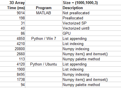
One thing you might notice is that the GPU isn't the fastest method for this situation. Using the GPU does not always guarantee that it will improve performance. Another thing is that using Numpy and standard indexing is painfully slow, even compared to non pre-allocated MATLAB arrays. MATLAB is certainly fast, pre-allocated MATLAB arrays are not much slower than Numpy's palette method (which is a form of vectorization). Although if you are stuck using Numpy then clearly using the item() and itemset() methods is faster than standard indexing, but it is even better if you can use the palette method. Additionally switching to the Ubuntu OS seems to improve Numpy's performance.
Scipy Weave lets you write C code right inside of your Python program. Cython is a little different but it also allows you to work with C code in Python. Because C is a slightly lower-level language than MATLAB and Python you might be able to get faster performance from C. However the truth is that when you vectorize your code you are essentially asking MATLAB and Python to turn your vectorized code into very efficient low-level algorithms. These algorithms are often faster than anything you could easily write yourself, but Weave can still be worth a try.
I'm not going to go into too much detail about these methods because I don't think that they are typically worth the effort. I had trouble getting Weave to work in Windows 7. In Ubuntu when it did work it was still slower than Numexpr in Windows 7.
When I first learned about Scipy Weave I figured that I would end up having to use that if I really wanted the best performance out of Python. Numexpr is so fast though that I've decided to not spend my time writing C code. Numexpr is essentially as easy to write as vecorization is. One downside to Numexpr is that the first time it runs a string of code it must first optimize and compile that code. Therefore the first time it may take around 100ms or so just before it actually runs the code. This compile time is not included in the chart below.
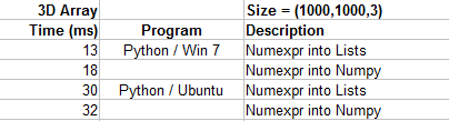
All four of these methods are better than any of the results in the previous chart. Although Numexpr is the fastest method in this test case, it will get beaten by a GPU in a more complex test case. Take a look at these results from this Bio-Engineering problem. Numexpr is the fastest CPU method, but the GPU can be much faster.
import numpy as np
import numexpr as ne
import time

# create the initial image of size 1000x1000 with random values 0, 1, or 2
s2 = 1000
img = np.random.randint(0,3,(s2,s2))
color = [0,0,0]

start = time.time()
q = [[],[],[]]
# Numexpr compliles the optimized code needed to run
# the expression that you input as a string.
q[0] = ne.evaluate("(img==0)*255")
q[1] = ne.evaluate("(img==1)*255")
q[2] = ne.evaluate("(img==2)*255")
elapsed = time.time() - start
print "Numexpr with Lists:", elapsed

start = time.time()
qq = np.zeros((3,s2,s2),np.uint8)
qq[0] = ne.evaluate("(img==0)*255")
qq[1] = ne.evaluate("(img==1)*255")
qq[2] = ne.evaluate("(img==2)*255")
elapsed = time.time() - start
print "Numexpr with Numpy:", elapsed